For European anchovy (Engraulis encrasicolus) in the Mediterranean Sea, do the largest local climatic changes occur where future conditions lie beyond the species’ estimated climatic range? This example compares the amount of change with its consequences for distance from the species’ average climate. It uses six Bio-ORACLE v3 surface variables under SSP2-4.5 and current location weights from a continuous presence-background SDM.
library(climniche)

case_path <- system.file("extdata/mediterranean_anchovy", package = "climniche")

case_cells <- read.csv(
  file.path(case_path, "anchovy_climniche_input_sample.csv"),
  check.names = FALSE
)
layer_manifest <- read.csv(
  file.path(case_path, "anchovy_biooracle_layer_manifest.csv")
)
sdm_settings <- read.csv(
  file.path(case_path, "anchovy_presence_background_sdm_settings.csv")
)
metric_weights <- read.csv(
  file.path(case_path, "anchovy_climniche_sensitivity_weights.csv")
)
Climatic data
The six retained variables describe temperature, salinity, pH and water movement. Current layers represent 2000-2019, except pH (2000-2018); future layers represent 2050. Current and future layers have identical variables, resolution and cell order.
variable_table <- subset(
  layer_manifest,
  retained_for_climniche,
  c("variable", "label", "depth", "current_time", "future_time")
)
variable_table[["future_scenario"]] <- "SSP2-4.5"
variable_table
#>                variable               label               depth
#> 1      temperature_mean    Mean temperature surface (depthsurf)
#> 2     temperature_range   Temperature range surface (depthsurf)
#> 3        salinity_range      Salinity range surface (depthsurf)
#> 5               ph_mean             Mean pH surface (depthsurf)
#> 6  sea_water_speed_mean  Mean current speed surface (depthsurf)
#> 7 sea_water_speed_range Current speed range surface (depthsurf)
#>                                  current_time          future_time
#> 1 Bio-ORACLE v3 baseline time layers averaged 2050-01-01T00:00:00Z
#> 2 Bio-ORACLE v3 baseline time layers averaged 2050-01-01T00:00:00Z
#> 3 Bio-ORACLE v3 baseline time layers averaged 2050-01-01T00:00:00Z
#> 5 Bio-ORACLE v3 baseline time layers averaged 2050-01-01T00:00:00Z
#> 6 Bio-ORACLE v3 baseline time layers averaged 2050-01-01T00:00:00Z
#> 7 Bio-ORACLE v3 baseline time layers averaged 2050-01-01T00:00:00Z
#>   future_scenario
#> 1        SSP2-4.5
#> 2        SSP2-4.5
#> 3        SSP2-4.5
#> 5        SSP2-4.5
#> 6        SSP2-4.5
#> 7        SSP2-4.5
The diagonal climatic metric uses the ratio of current-domain variance to occurrence-cell variance, bounded to 0.25-4 and normalised to mean one. These weights determine each variable’s contribution to climatic distance. They are separate from the location weights supplied by SDM suitability.
weight_table <- merge(
  variable_table[c("variable", "label")],
  metric_weights[c("variable", "sensitivity_weight")],
  by = "variable",
  sort = FALSE
)
names(weight_table) <- c(
  "Variable", "Climate variable", "Climatic metric weight"
)
weight_table
#>                Variable    Climate variable Climatic metric weight
#> 1      temperature_mean    Mean temperature              0.7709378
#> 2     temperature_range   Temperature range              0.9848117
#> 3        salinity_range      Salinity range              2.0457639
#> 4               ph_mean             Mean pH              0.7755083
#> 5  sea_water_speed_mean  Mean current speed              0.6458254
#> 6 sea_water_speed_range Current speed range              0.7771529
The package contains a 2,000-cell extract of the prepared raster inputs so that the central calculation runs when this vignette is built. The maps later in the vignette come from the full Mediterranean raster analysis.
climate_variables <- variable_table[["variable"]]
current_columns <- paste0(climate_variables, "_current")
future_columns <- paste0(climate_variables, "_future")

current_climate <- as.matrix(case_cells[current_columns])
future_climate <- as.matrix(case_cells[future_columns])
colnames(current_climate) <- climate_variables
colnames(future_climate) <- climate_variables

weight_row <- sdm_settings[["setting"]] == "sdm_threshold"
sdm_threshold <- as.numeric(sdm_settings[weight_row, "value"])
climatic_weights <- setNames(
  metric_weights[["sensitivity_weight"]],
  metric_weights[["variable"]]
)
Climate exposure relative to the current niche
The SDM cutoff was selected by maximising TSS on the held-out presence-background data. Suitability values at or below it receive zero location weight; values above it retain their continuous values.
# Retain suitability weights within the current modelled distribution.
anchovy_fit <- fit_climniche(
  current = current_climate,
  future = future_climate,
  occupied = case_cells[["sdm_suitability"]],
  occupied_threshold = sdm_threshold,
  sensitivity = climatic_weights,
  preprocess = FALSE
)

climniche_summary(anchovy_fit)
#>    Scope Cells Reference weight sum Boundary quantile Boundary distance
#>  current  1200             825.3044              0.95          5.241434
#>
#>                     Metric     Mean   Median 90th percentile
#>      Climatic Displacement 3.519480 3.509524       3.7255453
#>       Niche Distance Shift 2.184474 2.530491       2.9668506
#>   Climatic Reconfiguration 2.553753 2.376605       3.4869382
#>  Niche Boundary Exceedance 0.140777 0.000000       0.2373889
Climatic Displacement measures how much climate changes at each location. Niche Distance Shift shows whether conditions become closer to or farther from the weighted average climate. Climatic Reconfiguration retains changes not expressed as a distance shift, and Niche Boundary Exceedance measures how far future conditions extend beyond the estimated climatic range. The method example gives the definitions and a two-site comparison.
Mediterranean maps
The full raster workflow uses the same climatic variables and reference weights.
# Fit and map exposure within the Mediterranean study region.
spatial_fit <- fit_climniche_terra(
  current = current_layers[[climate_variables]],
  future = future_layers[[climate_variables]],
  occupied = anchovy_suitability,
  occupied_threshold = sdm_threshold,
  domain = mediterranean_sea_mask,
  sensitivity = climatic_weights,
  preprocess = FALSE
)

metric_maps <- plot_climniche_maps(
  spatial_fit,
  occupied = anchovy_suitability,
  occupied_only = TRUE,
  occupied_threshold = sdm_threshold,
  study_region = mediterranean_boundary,
  degree_labels = "hemisphere",
  legend_title = FALSE,
  legend_position = "bottom"
)

metric_maps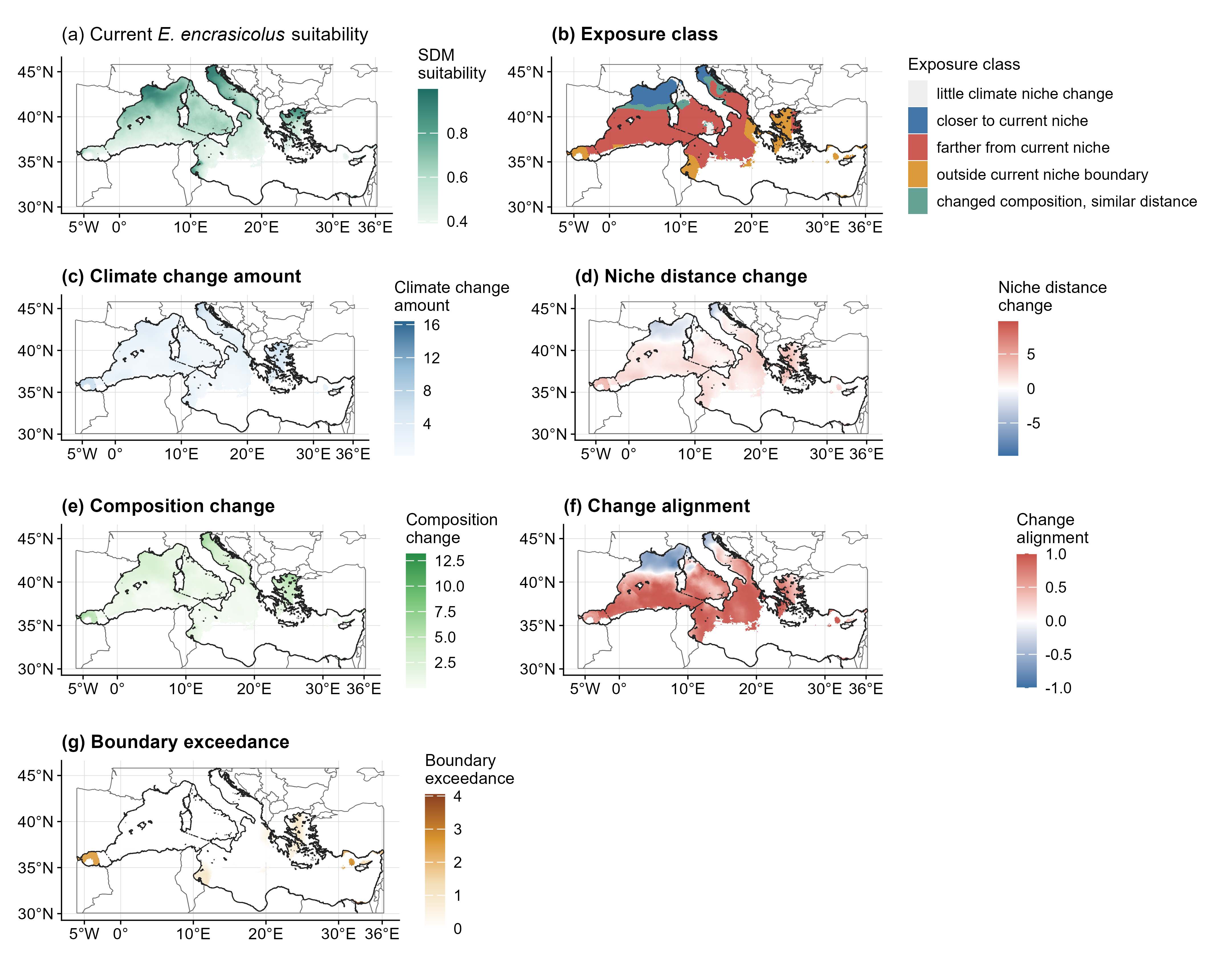
Summary figure
Panel (a) compares Climatic Displacement with Niche Distance Shift. Locations with similar amounts of change can move different distances towards or away from the average climate. Panel (b) compares Climatic Reconfiguration with Niche Boundary Exceedance. Panel (c) gives each variable’s weighted mean absolute share of the change in squared niche distance, rather than SDM variable importance. Panel (d) shows the weighted metric distributions.
variable_labels <- setNames(
  variable_table[["label"]],
  variable_table[["variable"]]
)

summary_figure <- plot_climniche_summary_figure(
  spatial_fit,
  scope = "current",
  top_variables = 6,
  variable_labels = variable_labels,
  title = NULL
)

summary_figure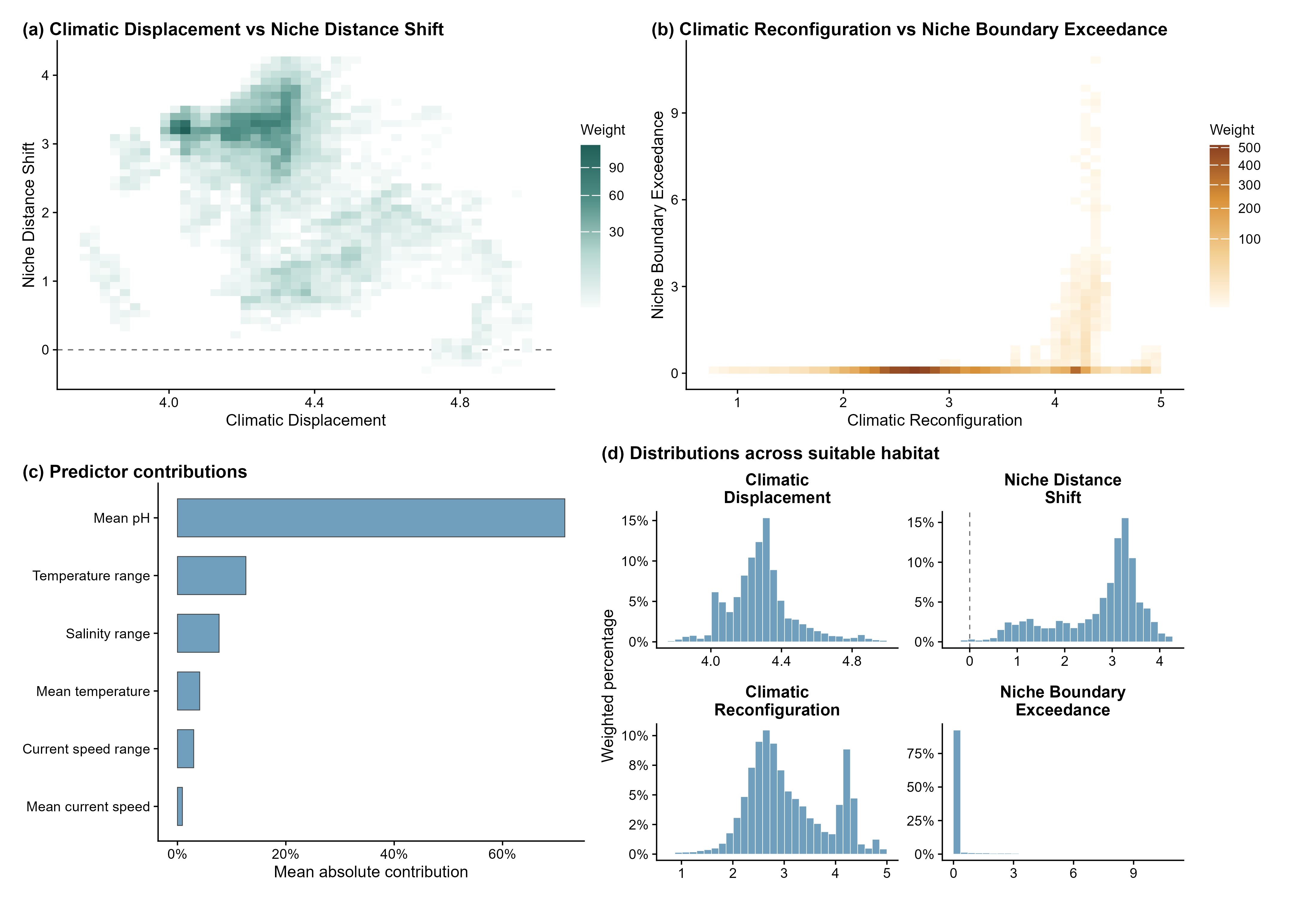
The exposure through time example applies the same fixed current niche reference to four SSP2-4.5 projections. The spatial climatic contribution example maps the cell-level pattern summarized in panel (c).
Data sources
Bio-ORACLE v3 layers follow Assis et al. (2024), Global Ecology and Biogeography 33, e13813. Occurrence records were obtained from the Ocean Biodiversity Information System. The study region uses Marine Regions IHO Sea Areas version 3 (doi:10.14284/323).