Exposure and habitat suitability

Where does high current habitat suitability coincide with climate moving away from the species’ average conditions? Where is local climate projected to change less? climniche_priority() compares an exposure quantity with habitat suitability to examine potential exposure hotspots and candidate climatic refugia within the current distribution.

Pareto screening

Each screen pairs one climniche quantity with one ecological criterion. A cell has Pareto rank 1 when no other retained cell is at least as preferred on both objectives and strictly preferred on one. Successive fronts describe increasing Pareto depth. The Pareto depth score rescales these fronts from zero to one, with one assigned to the non-dominated front.

Locations on the same front can trade a better value of one criterion for a poorer value of the other. The plot retains both criteria so those trade-offs can be inspected.

Mediterranean anchovy

The spatial fit is taken from the European anchovy example. Current SDM suitability provides the second criterion for both screens and also supplies the location weights defining the current climatic reference.

Potential exposure hotspots: prefer higher current suitability and a larger positive Niche Distance Shift. Positive values represent movement away from the weighted average climate.

positive_shift <- climniche_priority(
  spatial_fit,
  exposure = "niche_distance_change",
  criterion_name = "Current SDM suitability",
  scope = "current",
  positive_only = TRUE,
  exposure_direction = "maximize"
)

Potential climatic refugia: prefer higher current suitability and lower Climatic Displacement, favouring current habitat with comparatively little projected climatic change.

low_displacement <- climniche_priority(
  spatial_fit,
  exposure = "climate_change_amount",
  criterion_name = "Current SDM suitability",
  scope = "current",
  positive_only = FALSE,
  exposure_direction = "minimize"
)

Profile	Exposure	Direction	Ranked cells	Pareto fronts	First front
Positive Niche Distance Shift	Niche Distance Shift	maximize	13,495	265	18
Low Climatic Displacement	Climatic Displacement	minimize	13,584	212	30

Decision planes and maps

positive_shift_figure <- plot_climniche_priority(
  positive_shift,
  type = "both",
  map_value = "pareto_depth_score",
  study_region = mediterranean_boundary,
  degree_labels = "hemisphere"
)

low_displacement_figure <- plot_climniche_priority(
  low_displacement,
  type = "both",
  map_value = "pareto_depth_score",
  study_region = mediterranean_boundary,
  degree_labels = "hemisphere"
)

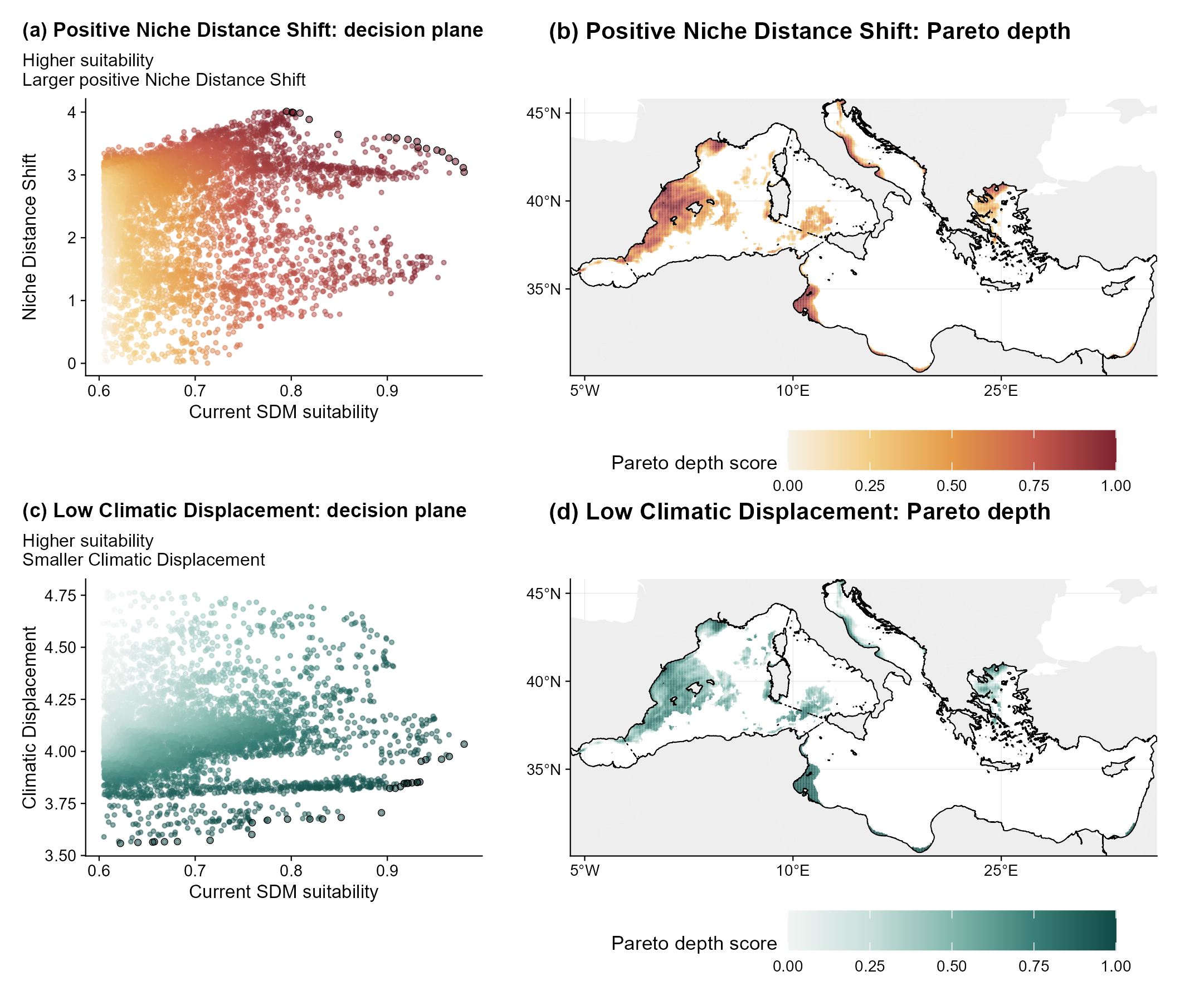
Panels (a) and (c) retain the two objectives and outline the first Pareto front. Panels (b) and (d) map the depth of each retained cell relative to its own screen. Pareto depth scores are therefore interpreted within a screen, not compared between the two maps.

Another quantity, such as abundance, habitat condition or management cost, can be supplied through criterion, with the preferred direction set by criterion_direction.

The Pareto procedure follows the spatial multi-criteria application of Tracey et al. (2018).