Two locations can experience the same climatic change yet reach
different conditions relative to a species’ current climate.
climniche measures both the amount of local change and
where that change takes each location.
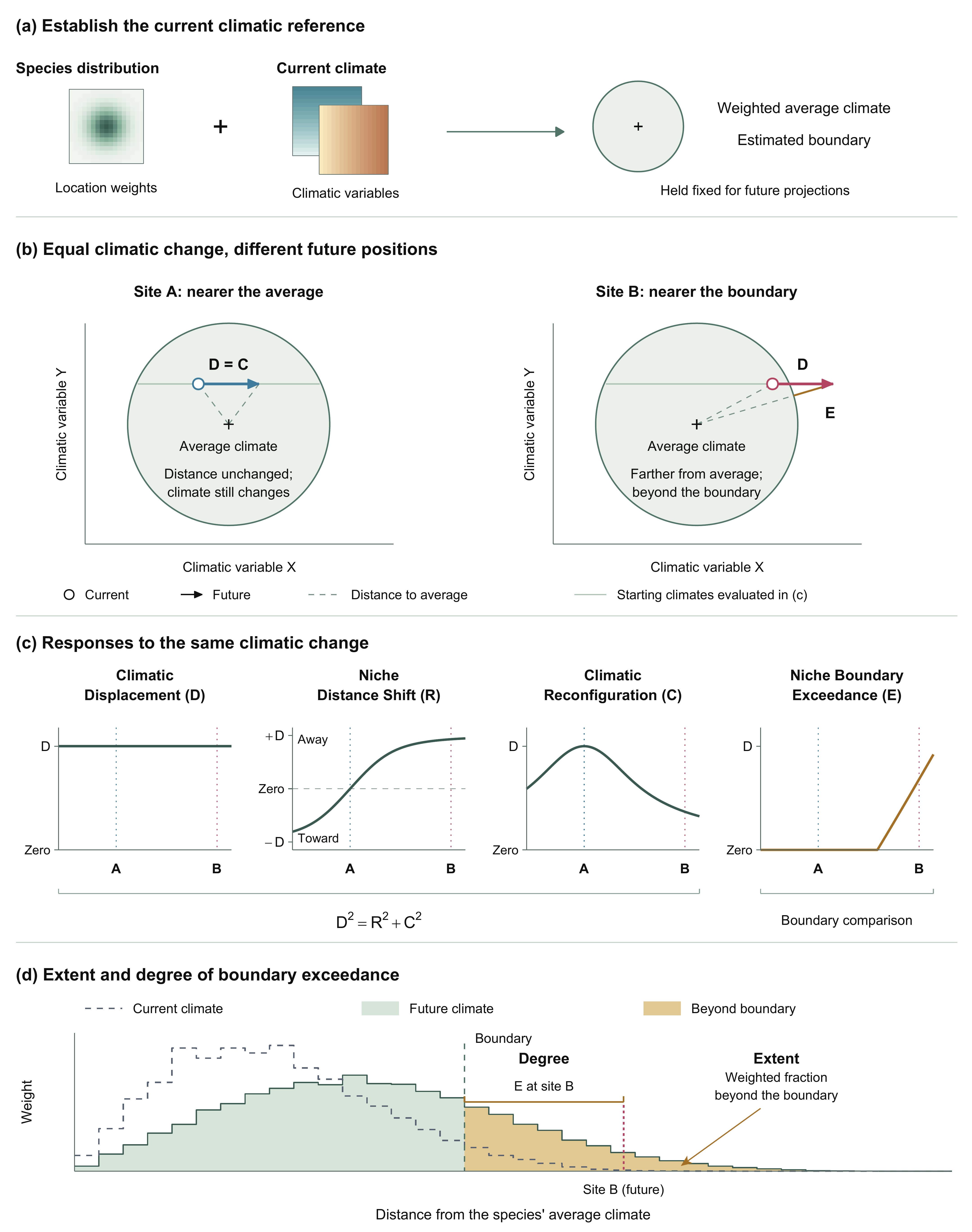
Equal climatic change, different exposure. (a) The current distribution and climate define the reference. (b) Identical displacements leave site A equally distant from the average climate but move site B beyond the boundary. (c) Metric responses vary with starting climate. (d) The gold area represents the weighted fraction beyond the boundary; the gold bracket shows the exceedance distance at site B. This is a conceptual example.
Define the current climatic reference
Species distribution data describe the climates associated with the
current range. climniche summarises this distribution of
climatic conditions by a weighted average and a radial boundary. This
empirical climatic niche reference is a proxy for the
species’ current climatic niche.
Each location receives a non-negative weight \(w_i\). Occurrence locations or locations
inside a binary distribution map receive weight one; other locations
receive zero. Continuous SDM suitability can supply continuous weights.
An optional occupied_threshold sets low values to zero
without changing the remaining values. With
occupied = NULL, all locations receive equal weight and the
reference describes the study region.
By default, near-constant variables and one variable at a time from highly correlated pairs are removed. Retained variables are standardised using unweighted current-climate means and standard deviations. The same variables and transformation are used for future climate.
Let \(c_i\) and \(f_i\) be the transformed current and future climatic vectors at location \(i\). The reference centre is
\[ \mu = \frac{\sum_i w_i c_i}{\sum_i w_i}. \]
Distance is measured under a symmetric positive semidefinite matrix \(A\):
\[ d_A(x,y) = \sqrt{(x-y)^\mathsf{T}A(x-y)}. \]
The location weights \(w_i\)
determine how locations contribute to the reference. The climatic
variable weights in \(A\) determine how
variables contribute to distance. Standardised variables have equal
weights by default; users can supply sensitivity or
A to change their relative contributions.
Writing \(r_{0i}=d_A(c_i,\mu)\), the boundary is
\[ B_q = Q_q^w(r_0). \]
For boundary = 0.95, at least 95% of the current
location weight lies at or within this distance. The boundary therefore
encloses an estimated climatic range, rather than every climatic
condition in the input data.
Compare current and future climate
The transformation, climatic variable weights, centre and boundary remain fixed when future conditions are evaluated.
Climatic Displacement measures the amount of local climatic change:
\[ D_i = d_A(f_i,c_i). \]
Niche Distance Shift measures change in distance from the weighted average climate. Negative values indicate movement towards the average and positive values indicate movement away:
\[ R_i = d_A(f_i,\mu)-d_A(c_i,\mu). \]
Climatic Reconfiguration captures the part of climatic displacement not expressed as a change in distance from the average:
\[ C_i = \sqrt{\max(0,D_i^2-R_i^2)}. \]
Different combinations of climatic variables can be equally distant from the average. When those distances are equal, Niche Distance Shift is zero and Climatic Reconfiguration equals Climatic Displacement, as at site A in the figure. These three quantities satisfy \(D_i^2=R_i^2+C_i^2\).
Niche Boundary Exceedance measures how far future conditions lie beyond the estimated range:
\[ E_i = \max(0,d_A(f_i,\mu)-B_q). \]
It is zero at or within the boundary and positive beyond it, as at site B. The comparison uses the future distance and the fixed boundary.
Reproduce the two-site comparison
The conceptual example uses two climatic variables with equal distance weights. A symmetric distribution of current climates defines the reference. The coordinates are already on a common scale, so no preprocessing or scaling is applied.
library(climniche)

# Define an illustrative current climatic distribution.
current <- as.matrix(expand.grid(
  climate_x = seq(-3, 3, length.out = 81),
  climate_y = seq(-3, 3, length.out = 81)
))
location_weights <- exp(-rowSums(current^2) / 2)

reference <- fit_climniche_reference(
  current,
  occupied = location_weights,
  A = diag(2),
  scale = FALSE,
  preprocess = FALSE,
  boundary = 0.95
)

# Apply the same climatic change at sites A and B.
boundary_distance <- reference[["boundary_distance"]]
current_sites <- boundary_distance * rbind(
  A = c(-0.30, 0.40),
  B = c(0.75, 0.40)
)
colnames(current_sites) <- colnames(current)
future_sites <- sweep(
  current_sites, 2, c(0.60 * boundary_distance, 0), "+"
)

site_fit <- project_climniche(
  reference,
  future = future_sites,
  current = current_sites
)

results <- climniche_table(site_fit, scope = "all")
site_metrics <- results[c(
  "climate_change_amount", "niche_distance_change",
  "climate_reconfiguration", "niche_boundary_exceedance"
)]
names(site_metrics) <- c(
  "Climatic Displacement", "Niche Distance Shift",
  "Climatic Reconfiguration", "Niche Boundary Exceedance"
)
knitr::kable(cbind(Site = c("A", "B"), site_metrics), digits = 3)| Site | Climatic Displacement | Niche Distance Shift | Climatic Reconfiguration | Niche Boundary Exceedance |
|---|---|---|---|---|
| A | 1.449 | 0.000 | 1.449 | 0.000 |
| B | 1.449 | 1.348 | 0.533 | 0.985 |
The two sites have identical Climatic Displacement. At site A, the climatic combination changes without a net change in distance. At site B, future conditions are farther from the average and outside the boundary.
From locations to the current distribution
The same projection can be applied to all reference locations. Their current weights are retained when summarising future conditions.
# Apply the same change throughout the reference distribution.
future <- sweep(current, 2, c(0.60 * boundary_distance, 0), "+")
distribution_fit <- project_climniche(reference, future)
climniche_range_summary(distribution_fit)
#>     scope    n aggregation_weight_sum boundary_distance
#> 1 current 6561                 1111.7          2.415186
#>   boundary_exceedance_tolerance exposed_fraction
#> 1                             0        0.2439863
#>   conditional_relative_exceedance range_wide_relative_exceedance
#> 1                       0.2254591                     0.05500893
#>   mean_niche_boundary_exceedance
#> 1                      0.1328568
The weighted fraction beyond the boundary describes the extent of exceedance. The conditional mean describes its degree among locations beyond the boundary. This distinction underlies panel (d).
Apply the workflow to a species
fit_climniche() fits the reference and evaluates one
future projection from matrices or data frames.
fit_climniche_raster() and
fit_climniche_terra() perform the same calculation for
raster and terra objects, respectively.
Climate rasters must share their grid and coordinate system. The spatial
functions apply the study-domain mask and return results on that
grid.
The Mediterranean example demonstrates these steps for European anchovy. Exposure through time uses one current reference across successive future projections.