How much of the current distribution experiences climate beyond its estimated range in successive projections, and does the degree of exceedance also increase? This example follows European anchovy (Engraulis encrasicolus) in the Mediterranean Sea at 2030, 2050, 2070 and 2090 under Bio-ORACLE SSP2-4.5.
Fit one climatic reference
The analysis uses the six Bio-ORACLE variables and the continuous anchovy SDM suitability layer prepared in the Mediterranean example. The empirical climatic niche reference is fitted once. Its centre, climatic variable weights and radial boundary are then held fixed across all four projections.
projection_years <- c(2030, 2050, 2070, 2090)

future_series <- list(
  ssp245_2030 = climate_2030,
  ssp245_2050 = climate_2050,
  ssp245_2070 = climate_2070,
  ssp245_2090 = climate_2090
)

# Compare all periods with the same current climatic reference.
series <- fit_climniche_series(
  current = current_climate,
  future = future_series,
  time = projection_years,
  scenario = "SSP2-4.5",
  occupied = anchovy_suitability,
  occupied_threshold = sdm_threshold,
  domain = mediterranean_sea_mask,
  sensitivity = climatic_weights
)
The order of the future list must match time. Current
and future rasters use the same variables, names, resolution and cell
alignment.
Range-level exposure
The summaries separate the extent of boundary exceedance from its
degree. Let \(E_{it}\) denote Niche
Boundary Exceedance for location \(i\)
at time \(t\) and \(B\) the fitted boundary distance. The
summary weight \(a_i=w_i s_i\) combines
the current suitability weight \(w_i\)
with raster cell area \(s_i\). With
boundary_exceedance_tolerance = 0,
\[ F_t = \frac{\sum_i a_i I(E_{it} > 0)} {\sum_i a_i} \]
is the Weighted Niche Boundary Exceedance Fraction,
\[ S_t = \frac{\sum_i a_i (E_{it}/B) I(E_{it} > 0)} {\sum_i a_i I(E_{it} > 0)} \]
is Conditional Relative Niche Boundary Exceedance, and
\[ M_t = \frac{\sum_i a_i (E_{it}/B) I(E_{it} > 0)} {\sum_i a_i} = F_t S_t \]
is Range Mean Relative Niche Boundary Exceedance. Here, \(I(\cdot)\) is the indicator function. Cell area affects these summaries but does not alter the location weights used to fit the climatic reference.
range_summary <- climniche_range_summary(
  series,
  scope = "current",
  area_weight = TRUE
)

subset(
  range_summary,
  select = c(
    time,
    exposed_fraction,
    conditional_relative_exceedance,
    range_wide_relative_exceedance
  )
)| Projection year | Weighted boundary exceedance fraction | Conditional relative Niche Boundary Exceedance | Range mean relative Niche Boundary Exceedance |
|---|---|---|---|
| 2030 | 7.7% | 27.6% | 2.1% |
| 2050 | 9.3% | 25.7% | 2.4% |
| 2070 | 28.4% | 15.3% | 4.3% |
| 2090 | 78.9% | 12.5% | 9.9% |
extent_plot <- plot_climniche_time(
  series,
  metric = "exposed_fraction",
  scope = "current",
  area_weight = TRUE,
  show_models = FALSE
)

conditional_plot <- plot_climniche_time(
  series,
  metric = "conditional_relative_exceedance",
  scope = "current",
  area_weight = TRUE,
  show_models = FALSE
)

range_plot <- plot_climniche_time(
  series,
  metric = "range_wide_relative_exceedance",
  scope = "current",
  area_weight = TRUE,
  show_models = FALSE
)

patchwork::wrap_plots(
  extent_plot,
  conditional_plot,
  range_plot,
  nrow = 1
)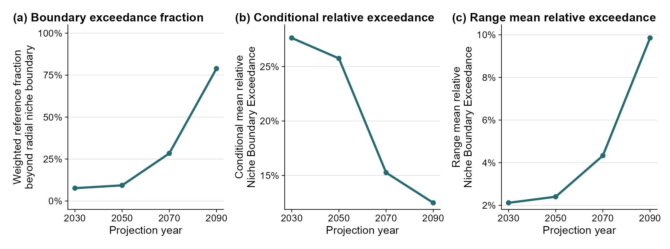
The suitability- and area-weighted fraction beyond the boundary increases from 7.7% in 2030 to 78.9% in 2090. Conditional Relative Niche Boundary Exceedance falls from 27.6% to 12.5% over the same period. Exceedance becomes more widespread even as its mean relative depth among locations beyond the boundary declines. Range Mean Relative Niche Boundary Exceedance, including zero values within the boundary, rises from 2.1% to 9.9%.
Timing within the current distribution
The first exceedance year identifies the first supplied projection in which a cell lies beyond the current niche boundary. The projection fraction records how many of the four supplied future periods exceed that boundary. Both summaries refer to the sampled projections and do not estimate an intervening crossing date.
departure <- climniche_departure(
  series,
  scope = "current"
)

rate <- climniche_change_rate(
  series,
  metric = "range_wide_relative_exceedance",
  scope = "current",
  area_weight = TRUE
)| Boundary exceedance fraction | Median first exceedance | Mean projection fraction |
|---|---|---|
| 78.9% | 2090 | 31.1% |
onset_map <- plot_climniche_departure_map(
  series,
  metric = "first_boundary_exceedance",
  scope = "current",
  scenario = "SSP2-4.5",
  study_region = mediterranean_boundary,
  degree_labels = "hemisphere"
)

frequency_map <- plot_climniche_departure_map(
  series,
  metric = "boundary_exceedance_projection_fraction",
  scope = "current",
  scenario = "SSP2-4.5",
  study_region = mediterranean_boundary,
  degree_labels = "hemisphere"
)

patchwork::wrap_plots(onset_map, frequency_map, nrow = 1)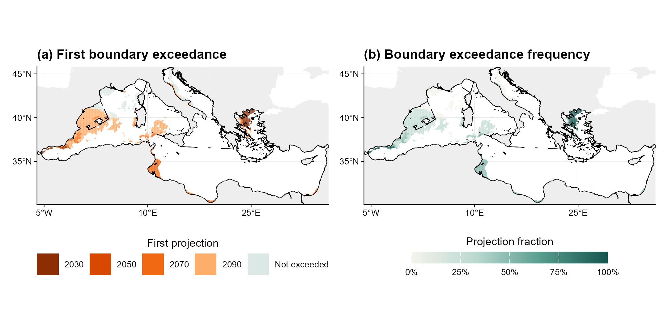
The map distinguishes early exceedance from cells whose future climate first appears beyond the boundary in 2090. The accompanying frequency map shows whether exceedance is confined to one projection or recurs across the series.
The largest increase in Range Mean Relative Niche Boundary Exceedance occurs between 2070 and 2090:
| Interval start | Interval end | Increase in range mean relative exceedance |
|---|---|---|
| 2070 | 2090 | 5.5 percentage points |
Report
climniche_series_report() collects the fixed niche
reference, projections, range summaries, temporal Niche Boundary
Exceedance summaries and interval changes.
series_report <- climniche_series_report(
  series,
  species = "European anchovy",
  scope = "current",
  area_weight = TRUE
)

series_report
write_climniche_series_report(
  series_report,
  "anchovy-exposure-through-time.md"
)