climniche

The places with the largest climatic changes need not be those where future conditions extend furthest beyond a species’ current climatic range. climniche measures local climate change alongside movement towards or away from the species’ average climate and the distance beyond its estimated climatic range.

Website: https://bohao0813.github.io/climniche/

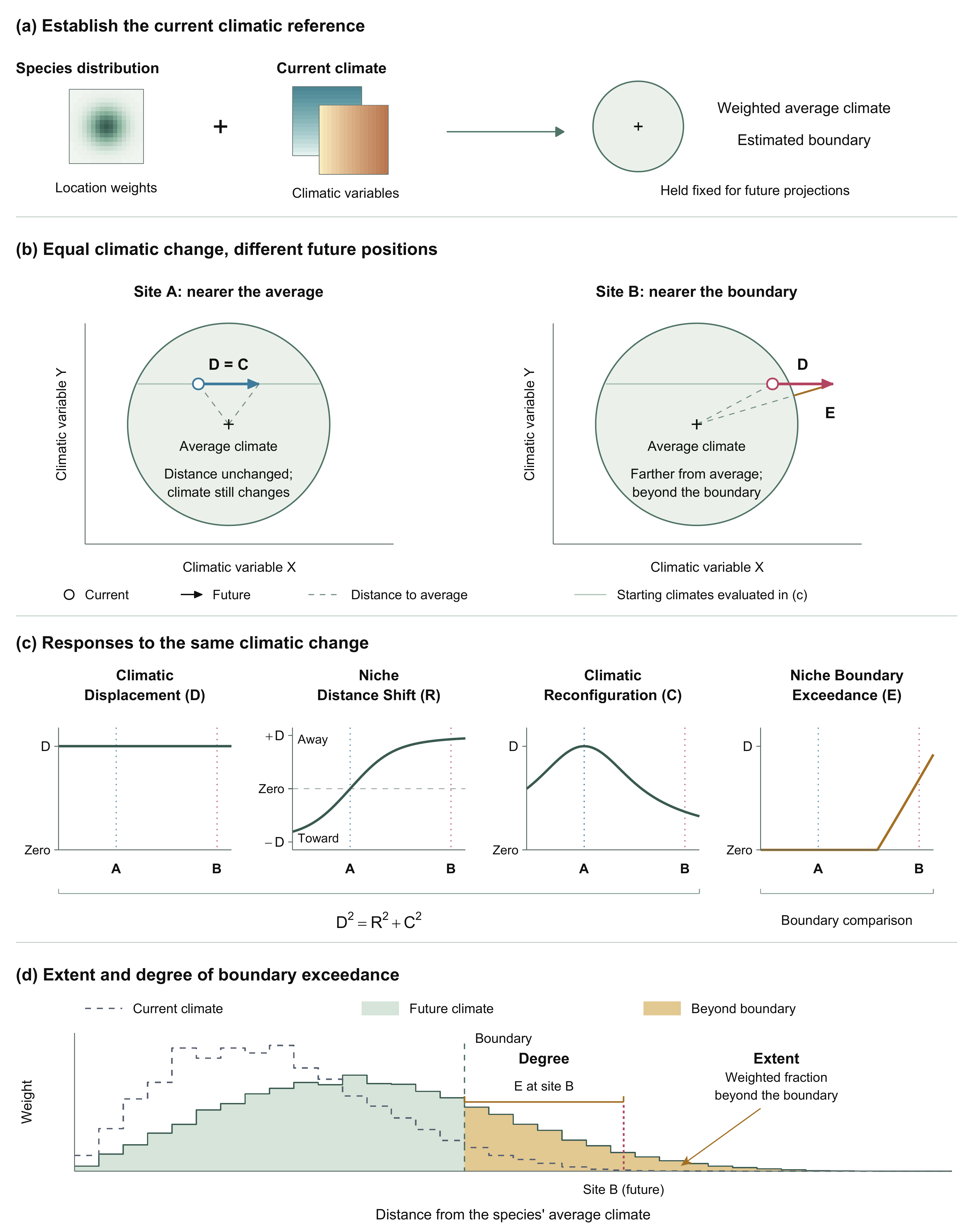
Equal climatic change, different exposure. A conceptual example calculated with climniche; calculation and interpretation.

Installation

Install the CRAN release:

install.packages("climniche")

Install the development version from GitHub:

install.packages("remotes")
remotes::install_github("Bohao0813/climniche")

What climniche measures

A species’ current distribution describes the climates it encounters. climniche summarises these conditions by a weighted average and an estimated climatic range, called the empirical climatic niche reference. This reference remains fixed when future conditions are evaluated.

• Climatic Displacement (climate_change_amount): the amount of climatic change at a location, measured as the distance between present and future climate.
• Niche Distance Shift (niche_distance_change): signed change in distance from the weighted average climate. Negative values indicate movement towards this average; positive values indicate movement away.
• Climatic Reconfiguration (climate_reconfiguration): the part of climatic displacement not expressed as a change in distance from that average.
• Niche Boundary Exceedance (niche_boundary_exceedance): the distance by which future conditions exceed the estimated climatic range. It is zero at or within the boundary.

Workflow

Every input interface follows the same four steps.

1. Supply present and future values of the same climatic variables at matching locations, together with species distribution data as location weights.
2. Remove near-constant and highly correlated variables, standardise the retained variables using current climate, and estimate the reference.
3. Keep the transformation, climatic variable weights, centre and boundary fixed while evaluating future conditions.
4. Extract results at each location, summarise the distribution, and draw maps or write reports.

fit_climniche() accepts numeric matrices and data frames. fit_climniche_raster() accepts RasterLayer, RasterStack and RasterBrick objects, whereas fit_climniche_terra() accepts SpatRaster objects. A fitted reference can also be created with fit_climniche_reference() and reused with project_climniche().

Basic use

library(climniche)

# Generate example climates and a current distribution.
sim <- simulate_climniche()

# Compare present and future conditions at the same locations.
fit <- fit_climniche(
  current = sim[["current"]],
  future = sim[["future_away"]],
  occupied = sim[["occupied"]],
  sensitivity = sim[["sensitivity"]]
)

# Summarise exposure within the current distribution.
climniche_summary(fit)
climniche_report(fit, species = "example species")
plot_climniche_summary_figure(fit)

Location weights can represent occurrence records, range maps, binary SDMs or continuous suitability. The raster interfaces accept binary and continuous reference rasters. occupied_threshold sets values at or below the cutoff to zero and retains larger values as continuous weights. domain limits the analysis to a study region; study_region adds its outline to maps.

Through time

fit_climniche_series() uses the same current climatic reference across future periods. This allows the extent and degree of boundary exceedance to be compared through time.

# Create four illustrative future projections.
future <- lapply(c(0.25, 0.50, 0.75, 1), function(fraction) {
  sim[["current"]] + fraction *
    (sim[["future_away"]] - sim[["current"]])
})

series <- fit_climniche_series(
  current = sim[["current"]],
  future = future,
  time = c(2030, 2050, 2070, 2090),
  occupied = sim[["occupied"]],
  sensitivity = sim[["sensitivity"]]
)

climniche_range_summary(series)
departure <- climniche_departure(series)
plot_climniche_time(series)

climniche_range_summary() separates how much of the weighted distribution lies beyond the boundary from how far those conditions extend beyond it. climniche_departure() records the first supplied projection beyond the boundary and the fraction of projections with exceedance. Consecutive runs can be examined with persistence.

Comparing exposure with habitat suitability

climniche_priority() compares one exposure quantity with habitat suitability or another ecological criterion. Two-objective Pareto ranking can help locate potential exposure hotspots or guide the search for climatic refugia.

The current location weight is the default second criterion. Supply criterion to use another quantity, such as abundance or habitat condition. The anchovy comparison pairs continuous SDM suitability with larger positive Niche Distance Shift or, in a separate analysis, with smaller Climatic Displacement. The output retains both criteria, Pareto ranks and mapped depth scores.

Climatic contributions

climniche_dominant_contribution() identifies the climate variable with the largest absolute contribution to squared niche distance change at each cell. Its dominance share measures how much of the total absolute contribution is assigned to that variable. These terms decompose the squared-distance change underlying Niche Distance Shift; they are not SDM variable importance.

contribution <- climniche_dominant_contribution(fit)
summary(contribution)

For a spatial fit, plot_climniche_dominant_contribution() maps the dominant variable and its share within the selected reference cells.

Worked example

The European anchovy example asks whether the largest climatic changes occur where future conditions lie beyond the species’ estimated climatic range in the Mediterranean Sea. Companion examples follow exposure from 2030 to 2090, identify climatic variables contributing to spatial differences, and compare exposure with habitat suitability.

Contributor

Contributions are welcome. Please make a pull request or contact bohao.he@polimi.it.